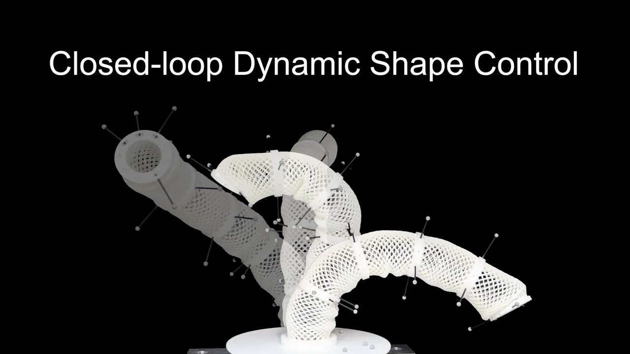
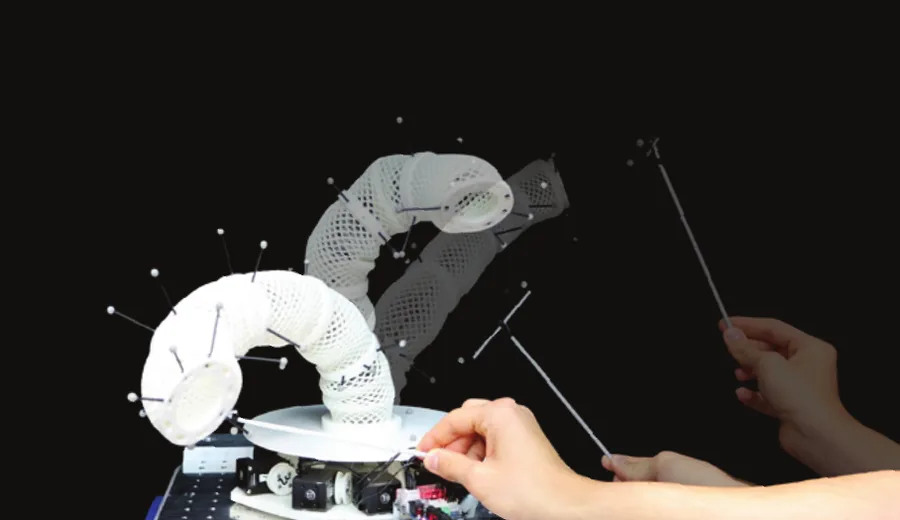
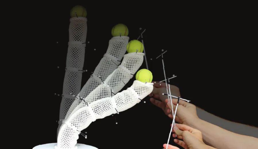
An adiabatic spectral submanifold (aSSM) model of the full body, learned from hardware data, lets model predictive control steer the whole shape of a soft trunk robot, not only its tip. With one six-dimensional model, the trunk settles into target shapes with ten times less error than with the best linear model, and balances a tennis ball while following a hand-held wand.
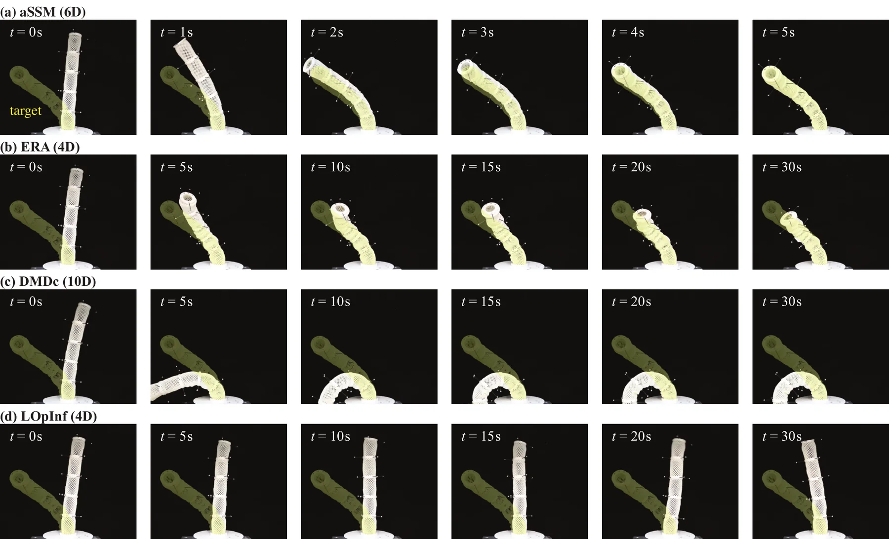
The motion-capture logs behind Fig. 4 and Table III, replayed from their timestamps, at 2× by default. Each controller starts from the relaxed trunk and has 30 s to bring bodies 1, 3 and 5 within 10 mm of their targets on average, and to hold them there for 4 s. Numbers on the cards are that mean distance, for the trunk as drawn. The trunk is drawn through the five tracked marker bodies; where motion capture loses or mislabels one, the drawing fills it in from nearby frames or from the bodies next to it.
Supplementary video
Whole-body shape control, on hardware.
Target shapes against three linear models, tennis-ball balancing (also tried with a model-free policy) and section-by-section shaping. Speed-ups are marked in the corner of each shot.
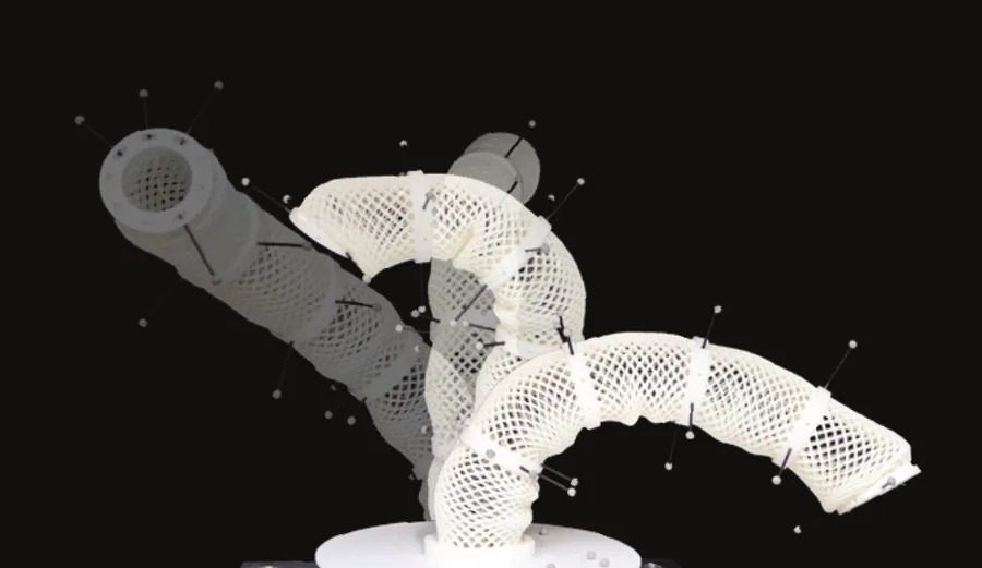
Fig. 1 Closed-loop full-body shape control of the five-segment trimmed-helicoid trunk, with earlier poses faded.
01 The robot
A trunk built to change shape.
Five trimmed-helicoid segments, 3D-printed in TPU, stack into a trunk 500 mm long and 170 g light. The compliance that gives it so many reachable shapes also makes the map from actuation to shape strongly nonlinear.
Three sections, nine tendons
Three tendons per section, 120° apart, bend it in two directions and contract it. Motion capture follows a marker body at the end of each segment; their positions and orientations form a 35-D pose.
Sleeves that bend the trunk
The upper sections’ tendons run through the segments below, in PTFE tubes. The tubes deform plastically after hours of use, and driving section 3 alone then bends the trunk below it by up to 58°.
Spring–tube sleeves
Nesting each tube in a closely wound extension spring keeps friction low while resisting the sleeve’s shortening. The largest uncommanded bend falls to 6°, and section 3 now bends 112° instead of 87°.
Fig. 2 Table I in the paper lists the tendon limits and deflections of both designs.
02 How it works
Learn the slow dynamics. Plan on them.
Soft robots move far more slowly than their own vibrations decay. Their dominant dynamics then lie on a low-dimensional manifold that drifts with the slowly changing input, an adiabatic spectral submanifold, and that manifold can be learned from data.
01
Record decays
The nine motors step through 20,000 static inputs from a Sobol sequence, and motion capture records how the trunk settles each time: 1.79 million samples at 100 Hz, just under five hours.
02
Map inputs to shapes
A radial-basis-function regression with 1,000 centres predicts the shape the trunk settles into for any input: the critical manifold.
03
Learn the aSSM
Delay-embedded decays around each settled shape are reduced to six coordinates. Quadratic polynomials map them back to the full 35-D pose and give their dynamics.
04
Plan with MPC
A sampling-based MPC scores three rounds of 1,000 candidate inputs against the model’s prediction and moves bodies 1, 3 and 5 toward their targets at 20 Hz.
One model, every task
The same 6-D model runs the aSSM controller in every task in the paper: target shapes, a moving shape, a hand-held wand, one section at a time and a ball on the tip. Each task changes only what the MPC is asked to do.
The theory, the delay embedding and the fits are in the paper’s Section III ↗.
03 On hardware
Three tasks on the real trunk.
Each model drives the same trunk through the same MPC. The baselines are linear models identified from the same data: the eigensystem realization algorithm (ERA), dynamic mode decomposition with control (DMDc) and Lagrangian operator inference (LOpInf), each at the reduced order that predicted best.
aSSM (6D)ERA (4D)DMDc (10D)LOpInf (4D)
From the supplementary video · aSSM at 1×, the linear models at 3×
The aSSM reaches every target, in 4.2 to 25.6 s, and then holds the shape with 5.1 mm mean error. The linear models cannot capture the nonlinearity that grows with large deflection: their error grows from base to tip, past 100 mm at the tip.
From the supplementary video · aSSM at 1×, sections 1 to 3 in turn
The inactive sections hold their shape while the active one is reshaped, and the standoff lets the operator both pull and push the trunk. ERA and DMDc also reach shapes the operator commands; LOpInf barely reacts.
From the supplementary video · aSSM, then all four; LOpInf at 2×
Under the aSSM the ball stays on for the whole run. ERA and DMDc hold neither the standoff nor the level and lose the ball within 2 s; LOpInf keeps it for 19.5 s only by leaving the trunk almost undeflected.
From the supplementary video · the trained PPO policy at 1×
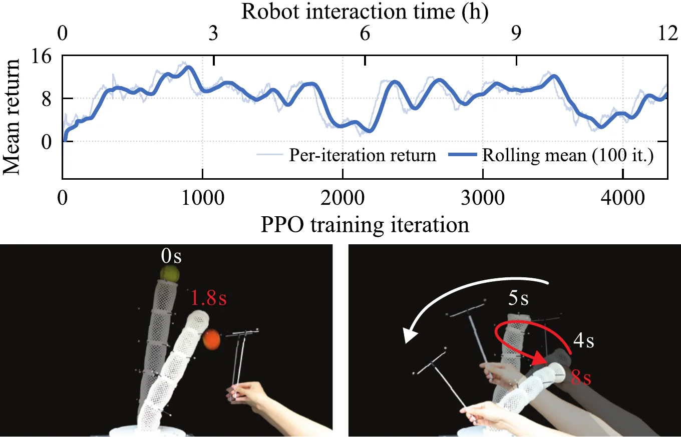
PPO, trained directly on the trunk for 4,320 iterations (4.3 million steps, 12 h of robot time), never finds a working policy: the return rises over the first 900 iterations and then oscillates. The trained policy follows the wand only over a small region, swings to the opposite side once the wand leaves it, and drops the ball after 1.8 s.
A sample-efficiency result, not a method comparison. Within 12 h on hardware the model-free policy found no working solution. The aSSM model came from 5 h of decay data and serves every task on this page.
04 Model and tracking
Prediction, and a moving shape.
Two more tests: predicting the trunk with no feedback at all, and following a shape that never stops moving.
Fig. 3Table II
7.5 s ahead, with no feedback
Rolled out from a single state for 750 steps, the aSSM keeps the tip within 27.5 mm on average, 2.9× closer than ERA. ERA damps the oscillations and settles to an offset, DMDc barely moves and LOpInf oscillates with growing amplitude.
Fig. 5Table IV
Dynamic shape tracking
A 30 s reference keeps all three sections bending and rotating and sweeps the tip by 167 mm. The aSSM follows it with 5.6 mm mean error per body and 2.6° in orientation, against 30.8 mm and 15.1° for ERA.
05 Paper
Read the paper.
Dynamic Shape Control of Soft Trunk Robots
Hehui Zheng, Marc Stampanoni, Roshan S. Kaundinya, Ronan Hinchet, George Haller, Robert K. Katzschmann
Controlling the shape profile of soft trunk robots extends their reach into complex regions of the workspace and enhances their use in practical applications. Recent advances in soft robot design have enabled soft trunk robots to achieve greater flexibility in conforming to complex shapes. Specifically, trunk robots whose geometries are designed as helicoids have been shown to enable extreme shape-changing capabilities. Their compliance makes them highly nonlinear, which in turn makes shape control difficult. On similar tendon-driven trunk robots, model-based controllers based on the theory of adiabatic spectral submanifolds (aSSMs) have achieved high accuracy in closed-loop end-effector tracking. We extend this approach by learning an aSSM model of the full body of a trimmed-helicoid soft trunk robot from data and use this in a model predictive control (MPC) scheme to demonstrate a range of shape control tasks on hardware. On closed-loop dynamic shape regulation, our method outperforms the available linear baselines by a factor of 10. In human-in-the-loop interactive demos, our method completes section-by-section shaping and balances a tennis ball for over 25 seconds, while the linear baselines fall short. A model-free reinforcement learning policy trained for 12 hours on hardware fails on the same balancing task. These results establish aSSM-based MPC as a practical route to full-body shape control on real soft hardware.
Citation
@misc{zheng2026dynamicshapecontrolsoft,
  title         = {Dynamic Shape Control of Soft Trunk Robots},
  author        = {Hehui Zheng and Marc Stampanoni and Roshan S. Kaundinya and
                   Ronan Hinchet and George Haller and Robert K. Katzschmann},
  year          = {2026},
  eprint        = {2611.06625},
  archivePrefix = {arXiv},
  primaryClass  = {cs.RO},
  url           = {https://arxiv.org/abs/2611.06625}
}